n-th Fibonacci Number: Recursion vs. Dynamic Programming

In this article, we will learn the concepts of recursion and dynamic programming by the familiar example which is finding the n-th Fibonacci number. Also at the same time, we will discuss the efficiency of each algorithm, recursive and dynamic programming in terms of time complexity to see which one is better.

Recursion

What is recursion?

Recursion in computer science is a method of solving a problem where the solution depends on solutions to smaller instances of the same problem. The approach can be applied to many types of problems, and recursion is one of the central ideas of computer science. Generally, recursion is the process in which a function calls itself directly or indirectly and the corresponding function is called a recursive function. I will examine the typical example of finding the n-th Fibonacci number by using a recursive function.

What is the Fibonacci sequence?

In mathematics, the Fibonacci sequence is the sequence in which the first two numbers are 0 and 1 and with each subsequent number being determined by the sum of the two preceding ones. That is

and

for n > 1

The Fibonacci sequence might look like this (the first 0 number is omitted):

1, 1, 2, 3, 5, 8, 13, 21, 34, 55, 89, 144, …

Find the n-th number in the Fibonacci sequence

Given a number n, write a program that finds the corresponding n-th Fibonacci Number. For example:

Input: n = 2
Output: 1

Input: n = 3
Output: 2

Input: n = 7
Output: 13

Now, we write a program to find the n-th number by using recursion (naive recursive algorithm) in JavaScript:

function nthFibonacci(n) {
    if (n < 2) { // if n < 2, then return its value
        return n;
    } else {
        return nthFibonacci(n - 1) + nthFibonacci(n - 2) // calling function recursively until reach the certain condition.
    }
}
nthFibonacci(7) // 13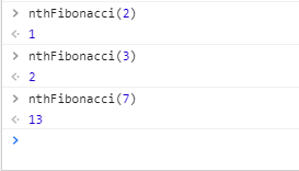

In Windows, press F12 or Ctrl + Shift + J to open the dev console to run this code above (Cmd + Option + J in MacOS).

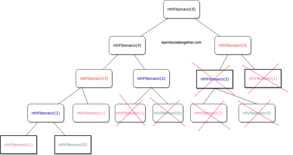
In this code above, we defined a function called nthFibonacci, which took n as an input and return the n-th number in the Fibonacci sequence. Inside this function, first we check if the input is smaller than 2 or not, if it’s we simple just return this number, otherwise we use the recursive function to make the function call itself repetitively until the input is less than 2. Here is what happened in this function, presume we typed 5 as an input, the recursive diagram should look like this:

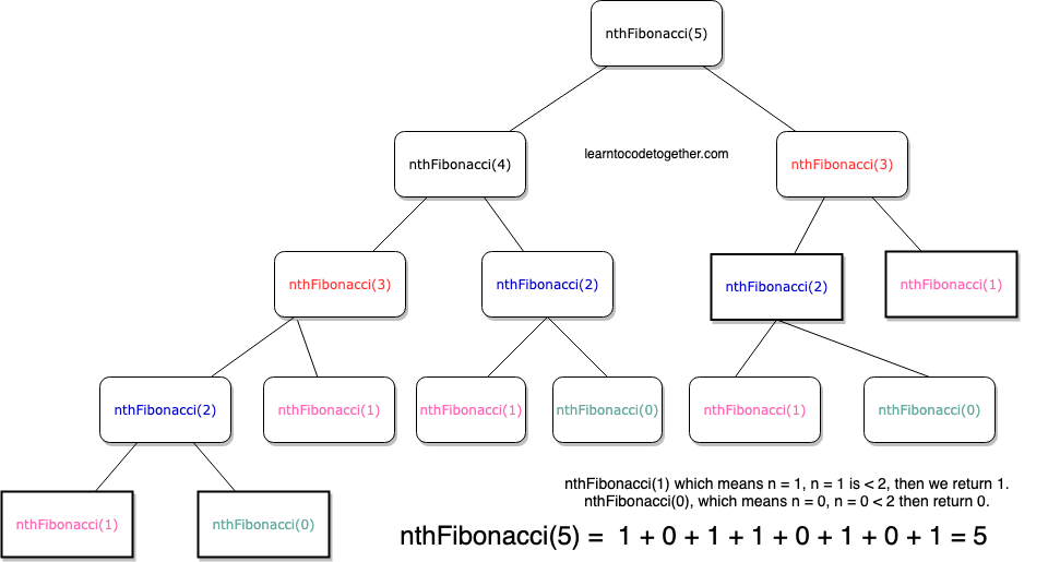
In order to find the 5th number, by looking back to the code above, because 5 is greater than 2, then nthFibonacci(5) = nthFibonacci(4) + nthFibonacci(3), but with nthFibonacci(4) and nthFibonacci(3) which are still larger than 2, then the process of recursing will be continued until the condition is reached. We can observe how it works by this diagram above, but for better understanding, look at the following things below:

nthFibonacci(5) = nthFibonacci(n - 1) + nthFibonacci(n - 2)
nthFibonacci(5) = nthFibonacci(4) + nthFibonacci(3)
Then we have:
nthFibonacci(4) = nthFibonacci(3) + nthFibonacci(2)
nthFibonacci(3) = nthFibonacci(2) + nthFibonacci(1)
so,
nthFibonacci(5) = (nthFibonacci(3) + nthFibonacci(2)) + (nthFibonacci(2) + nthFibonacci(1))
The function then further recursively:
nthFibonacci(3) = nthFibonacci(2) + nthFibonacci(1)
nthFibonacci(2) = nthFibonacci(1) + nthFibonacci(0)
then,
nthFibonacci(5) = (nthFibonacci(2) + nthFibonacci(1)) + (nthFibonacci(1) + nthFibonacci(0)) + (nthFibonacci(1) + nthFibonacci(0) + nthFibonacci(1))
The function again calls itself to resolve to nthFibonacci(2), it would not do the same thing with nthFibonacci(1) and nthFibonacci(0) because the value of n which are 1 and 0 is less than 2:
nthFibonacci(5) = ((nthFibonacci(1) + nthFibonacci(0)) + nthFibonacci(1)) + (nthFibonacci(1) + nthFibonacci(0)) + (nthFibonacci(1) + nthFibonacci(0) + nthFibonacci(1))
Now, after a lot of recursions, we finally reach the result as the diagram corresponding to the tree structure showed above. For simplifying, I write nthFibonacci(5) as f(5):
f(5) = f(1) + f(0) + f(1) + f(1) + f(0) + f(1) + f(0) + f(1) = 1 + 0 + 1 + 1 + 0 + 1 + 0 + 1 = 5

Hopefully, those things I wrote above make sense and now you understood how recursion works in finding the Fibonacci number.

The time complexity of n-th Fibonacci number using Recursion

When measuring the efficiency of an algorithm, typically we want to compute how fast is it algorithm with respect to time complexity. By using the recursive function, we can easily find out the n-th Fibonacci number, it is a proper algorithm, but is it considered a good algorithm? Definitely no. I changed the color of each function in the diagram on purpose, as you can see, the nthFibonacci(3) repeated 2 times, nthFibonacci(2) repeated 3 times, 5 times for nthFibonacci(1) and 3 times for nthFibonacci(0). Due to a lot of repeated work, the time to execute this function would be increased.

In the diagram, after each time the function decrement, the function gets double bigger until it reaches 1 or 0. The time complexity of this algorithm is:

2^0=1                        n
2^1=2            (n-1)                 (n-2)
2^2=4        (n-2)    (n-3)      (n-3)     (n-4)
2^3=8   (n-3)(n-4) (n-4)(n-5) (n-4)(n-5) (n-5)(n-6)
...
2^n-1

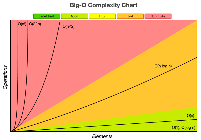
$T(n) = T(n - 1) + T(n -2) + 1 = 2^n = O(2^n)$ . This algorithm grows as exponential. The time complexity of this algorithm is labeled as horrible, according to this chart:

Dynamic Programming – Memoinization

Finding the n-th Fibonacci number with recursion it could be horrible when the input is large, the time wastes for this calculation could be unacceptable. The are many other alternative solutions to find the n-th Fibonacci number, including a technique called Dynamic Programming, the idea of this approach is simple to avoid the repeated work and store the sub-problems result so you don’t need to calculate it again.

What is dynamic programming?

Dynamic programming is both a mathematical optimization method and a computer programming method. The method was developed by Richard Bellman in the 1950s and has found applications in numerous fields. It’s the technique to solve the recursive problem in a more efficient manner. Many times in recursion we solve the problem repeatedly, with dynamic programming we store the solution of the sub-problems in an array, table or dictionary, etc…that we don’t have to calculate again, this is called Memoization. Simply put, dynamic programming is just memoization and re-use solutions.

In order to determine whether a problem can be solved in dynamic programming, there are 2 properties we need to consider:

Overlapping Subproblem
Optimal Structure

If the problem we try to solve has those two properties, we can apply dynamic programming to address it instead of recursion.

Overlapping sub-problems

As the name suggests, in recursion, overlapping sub-problems is when we calculate the same sub-problems over and over again. Instead of this redundant work, in dynamic programming, we solve the sub-problems only once and store those results for the latter use.

Now you see this tree structure again, with recursion, there are many times we had to re-calculate the sub-problems.

Optimal Structure

If the problem can be solved by using the solution of its sub-problems we then say this problem has optimal structure. This property is used to determine the usefulness of dynamic programming and greedy algorithms for a problem.

There are usually 7 steps in the development of the dynamic programming algorithm:

Establish a recursive property that gives the solution to an instance of the problem.
Develop a recursive algorithm as per recursive property
See if the same instance of the problem is being solved again an again in recursive calls
Develop a memoized recursive algorithm
See the pattern in storing the data in the memory
Convert the memoized recursive algorithm into an iterative algorithm (optional)
Optimize the iterative algorithm by using the storage as required (storage optimization)

Finding n-th Fibonacci Number with Dynamic Programming

Finding n-th Fibonacci number is ideal to solve by dynamic programming because of it satisfies of those 2 properties:

First, the sub-problems were calculated over and over again with recursion.
Second, we can solve the problem by using the result of its sub-problems.

There are 2 approaches in Dynamic Programming:

Bottom-up
Top-down

Bottom-up Approach – Tabulation

Presume we need to solve a problem for N, we start with the smallest possible input and that solution for future use. By doing that, you can use the stored solution to calculate the bigger problem.

In the Fibonacci example, if we have to find the n-th Fibonacci number then we will start with the two smallest value which is 0 and 1, then gradually we can calculate the bigger problems by re-use the result, here is the code example for finding the n-th Fibonacci number using Dynamic Programming with the bottom-up approach:

function nthFibDP(n) {
    let memo = new Array(n + 1);
    memo[0] = 0;
    memo[1] = 1;
    for (let i = 2; i <= n; i++) {
        memo[i] = memo[i - 1] + memo[i - 2];
    }
    return memo[n];
}
nthFibDP(6) // 8

Let’s break down to see what happened:

First, inside the nthFibDP function, we create a new array in order to store the solution of the sub-problems, and the size of this array is n + 1 because we spent the first index for the 0 number.
In the first two indices 0 and 1, the value of each index is 0 and 1 respectively.
Then we generated a loop that iterated from 2 to n (including n), inside that loop, by the bottom-up approach we calculate the smaller values then increase 1 bigger after each iteration by calculating the two preceding ones of this index, if the values of two preceding indices already exist in the array, then we use those values otherwise we have to calculate.
Because all the sub-problems’ solution were stored in the memo array, so the last element of this array was our solution, which led to why return memo[n].

And hereby is the explanation of the bare words, looks much like pseudocode:

n = 6;
f[0] = 0
f[1] = 1
f[] = [0, 1, x5 empty] (because n + 1)
for(i = 2; i <= 6; i++) (i <= n, n = 6)
      f[2] =  f[1] + f[0]
      f[2] = 1 + 0 = 1 (push the result to the correspon index)
      f[] = [0, 1, 1, x4 empty] (after adding f[2])

      f[3] = f[2] + f[1] (we just find the solution for f[2] = 1)
      f[3] =  1 + 1 = 2 (push the result to the 3rd index)
      f[] = [0, 1, 1, 2, x3 empty] (after adding f[3])

      f[4] = f[3] + f[2] (we just find the solution for f[3] = 2)
      f[4] =  2 + 1 = 3 (push the result to the 4rd index)
      f[] = [0, 1, 1, 2, 3, x2 empty] (after adding f[4])
      
      f[5] = f[4] + f[3] (we just find the solution for f[4] = 3)
      f[5] =  3 + 2 = 5 (push the result to the 5rd index)
      f[] = [0, 1, 1, 2, 3, 5, x1 empty] (after adding f[5])

      f[6] = f[5] + f[4] (we just find the solution for f[5] = 5)
      f[6] =  5 + 3 = 8 (push the result to the 6rd index)
      Now the array is: f[] = [0, 1, 1, 2, 3, 5, 8] (after adding f[6])

      Return f[n] <=> f[6]  = 8

To take a closer look, in your browser, open the console following keystroke F12 or Ctrl + Shift + J on Windows and Cmd + Option + J on macOS, paste the JavaScript code above to the console and add the keyword debugger inside your function and hit enter:

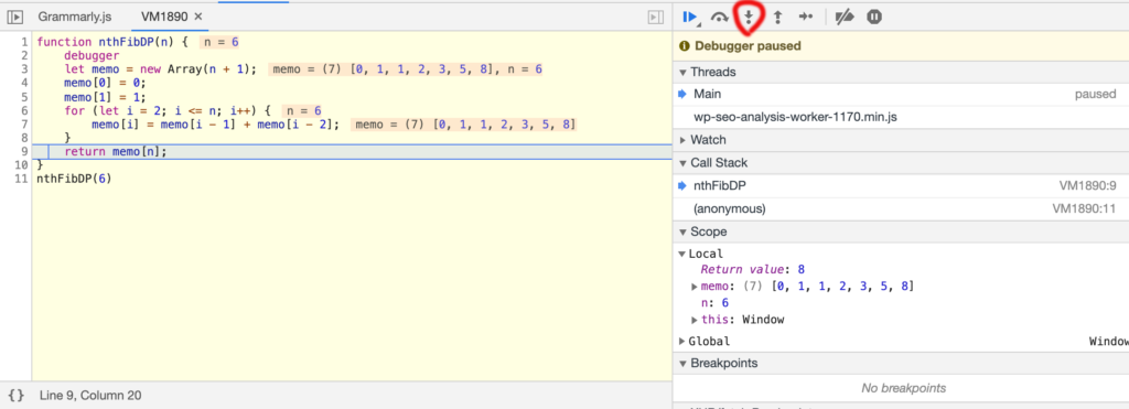
You can see in detail how this function is run by clicking to the arrow down symbol that I highlighted inside the circle red color.

Top-down Approach – Memoization

While the bottom-up approach starts with the smallest input and stores it for the future use to calculate the bigger one. Instead, top-down breaks the large problem into multiple subproblems from top to bottom, if the sub-problems solved already just reuse the answer. Otherwise, solve the subproblem and store the result. The top-down approach uses memoization to avoid recomputing the sub-problems.

Let’s let us again write n-th Fibonacci number by using the top-down approach:

function topDownFibonacci(n) {
    // pretty much like bottom-up, first create the array to keep the fibonacci numbers
    let saveF = new Array(n + 1);
// if n > 0, return value at this index
    if (saveF[n] > 0) return saveF[n];
    if (n <= 1) return n;
    // Recursion
    saveF[n] = topDownFibonacci(n - 1) + topDownFibonacci(n - 2)
    return saveF[n];
}
topDownFibonacci(7) // 13

This top-down approach looks much like the recursion method, but instead of re-computing a lot of sub-problems, we store the sub-problems we already compute in an array, and every sub-problems just need to be calculated once and can be reused for later calculation.

As you can see, a lot of repeated works have been eliminated hence save more time and space. You might wonder, you still can see some of the sub-problems repeated but remember, those problems just compute once and being reused.

The time complexity of Dynamic Programming

Both bottom-up and top-down use the technique tabulation and memoization to store the sub-problems and avoiding re-computing the time for those algorithms is linear time, which has been constructed by:

Sub-problems = n

Time/sub-problems = constant time = O(1)

Time complexity = Sub-problems x Time/sub-problems = O(n)

Comparing linear time with the exponential time of recursion, that is much better, right?

By the way, there are many other ways to find the n-th Fibonacci number, even better than Dynamic Programming with respect to time complexity also space complexity, I will also introduce to you one of those by using a formula and it just takes a constant time O(1) to find the value:

F_n = {[(√5 + 1)/2] ^ n} / √5

function nthFibConstantTime(n) {
    let phi = (1 + Math.sqrt(5)) / 2;
    return Math.round(Math.pow(phi, n) / Math.sqrt(5));
}
nthFibConstantTime(9) // 34

TL; DR

Recursion is a method to solve problems by allowing function calls itself repeatedly until reaching a certain condition, the typical example of recursion is finding the n-th Fibonacci number, after each recursion, it has to calculate the sub-problems again so this method lacks efficiency, which has time complexity as $O(2^n)$ (exponential time) so it’s a bad algorithm. Hence, another approach has been deployed, which is dynamic programming – it breaks the problem into smaller problems and stores the values of sub-problems for later use. To determine whether a problem can be solved with dynamic programming we should define is this problem can be done recursively and the result of the sub-problems can help us solve this problem or not. Dynamic programming is not something fancy, just about memoization and re-use sub-solutions. 2 techniques to solve programming in dynamic programming are Bottom-up and Top-down, both of them use $O(n)$ time, which is much better than recursion $O(2^n)$ . There are also many ways to solve the n-th Fibonacci number problem, which just takes $O(log N)$ or $O(1)$ .

Facebook0 Tweet0

n-th Fibonacci Number: Recursion vs. Dynamic Programming13 min read