Graph and its representation - Learn To Code Together

Graph Description

In this article, we will learn about what is a Graph and also its representation in computer science. After reading this article, you’ll be able to understand what graph is and some fundamental concepts around it. If you want to stick with learning algorithms for a long time, understanding the graph is essential and should be got accustomed to early. This is a crucial concept to learn because many algorithms today are used and implemented by using graphs, some of those will appear in the next article.

A graph is a data structure that consists of a finite set of vertices, and also called nodes, each line connecting vertices we call it an edge. The edges of the graph are represented as ordered or unordered-pairs, depending on whether the graph is directed or undirected.

More formally, in mathematics, and more specifically in graph theory, a graph is a structure amounting to a set of objects in which some pairs of the objects are in some sense “related”. The objects correspond to mathematical abstractions called vertices (also called nodes or points) and each of the related pairs of vertices is called an edge.

Graphs are used to solve many real-life problems. Graphs are used to represent networks. The networks may include paths in a city or telephone network or circuit network, solving Rubik’s cube. Graphs are also used in social networks like LinkedIn, Facebook. For example, on Facebook, each person is represented with a vertex(or node). Each node is a structure and contains information like person id, name, gender, locale, etc.

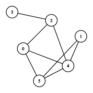
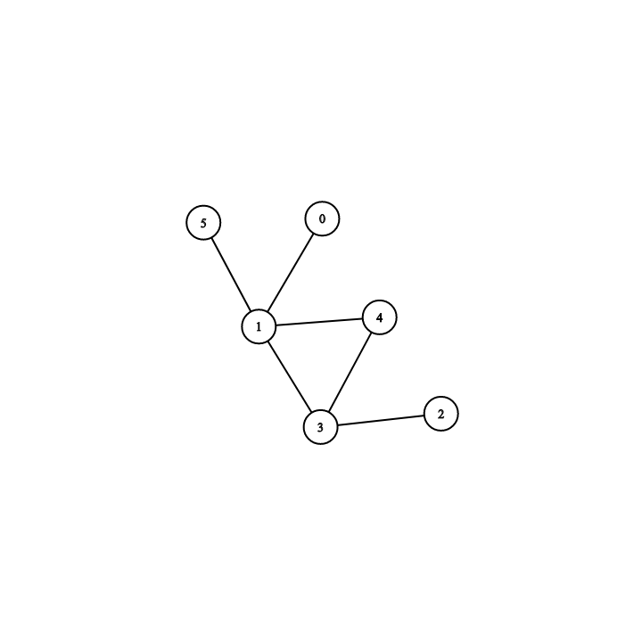
In those 2 graphs above, we can see totally a set of 6 vertices (6 nodes), which represent 6 numbers 0, 1, 2, 3, 4, 5, if you want to talk about one of those vertices on the graph, such as 1, we call it a vertex. We also can see several edges which connect vertices here, for example in the undirected graph, let’s count the total vertices and edges in this graph:

V = {0, 1, 2, 3, 4, 5}
E = {{0, 4}, {0,5}, {0, 2}, {1, 5}, {1, 4}, {2,4}, {3,2}, {4,5}}

We usually denote a set of edges as E and a set of vertices as V. We see that the undirected graph’s edges, represented by E, have no order to them since it’s possible to travel from one vertex to the other which mean we can say, for example, {0,4} equals to {4,0}. For general if we denote an edge connecting vertices $u$ and $v$ by the pair $(u,v)$ , then $(u,v)$ and $(v,u)$ have no difference. An edge between two vertices, such as the edge between 1 and 5, is incident on the two vertices, and we say that the vertices connected by an edge are adjacent or neighbors. The number of edges incident on a vertex is the degree of the vertex.

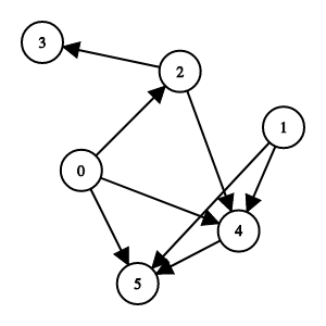
However, in the edge set E for the directed graph, there is the directional flow that’s important to how the graph is structured, and therefore, the edge set is represented as ordered pairs like this:

E = {(0, 4), (0,2), (0,5), (1, 4), (1, 5), (2, 3), (2, 4)}

We easily can distinguish the difference between the undirected graph and directed graph in which each edge goes both ways and we don’t see a direction, or we don’t see an arrow. But in the directed graph, we can see the arrows which indicate the direction of the edges and don’t necessarily go both ways.

Back to the undirected graph above, from vertex number 1 how many ways that we can go to get to the vertex number 5? As you can see, there are several ways. You can go from 1 then 4 then finally 5. Or you want to traverse more before reaching the final vertex that means you go from 1 then go to 4 then 0 then finally 5. But go through 1 to 5 is the fastest way. We call each the ways of this procedure as a path and go through 1 to 5 is the shortest path in which we just have to traverse 2 edges, two first approaches that go from 1 to reach 5 are not considered as shortest paths because they required more traversal between edges than the last approach.

When a path goes from a particular vertex back to itself, we call it a cycle. A graph may contain many cycles. We see one of them here, starting with the vertex number 0 -> 1 -> 2 -> 3 -> 4 -> 5 then go back to 0:

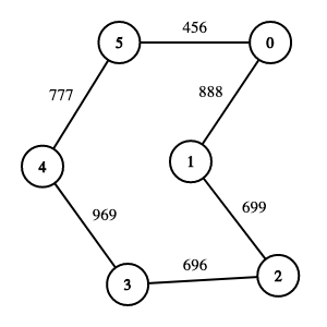
We also can see something new here, there are some numbers put on edges, we call those numbers as the weight of those edges and for a graph whose edges have weights is a weighted graph. Pay attention back to the first two images, we can see that there is no number in edges, so those graphs are unweighted-graph with no weight in edges.

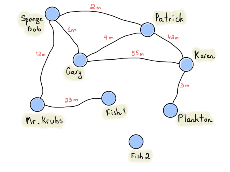
In the case of a road map, if you want to find the shortest route between two locations, you need to find out a route between two vertices which has the minimum sum of edge weights over all paths between the two vertices. Presume that we want to go from Sponge to Plankton, the shortest path here is we go from Sponge to Patrick then Karen finally to Plankton with the total distance is 48 miles.

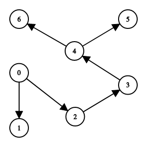
Now look at the image above, have you notice that there is no cycle in this unweighted directed graph, for those particular graphs like this, we call it directed acyclic graph or dag for short. We say that a directed edge leaves one vertex and enters another, as you can see with the vertex number 4, there is an edge that one vertex enters to 4, which is 3, and there are 2 vertices from 4 point to, which are 5 and 6. We call the number of edges leaving is its out-degree and in-degree with the number of edges entering the vertex.

Graph representation

After absorbing a lot of different terminologies. Now is the time for us to…relax, just kidding, wonder how can we represent those graphs in some specific ways. Actually there are some ways to handle such a thing but each of them all has its advantages and disadvantages. And three most common ways to represent a graph are Edge lists, Adjacency matrices, and Adjacency lists.

As mentioned above, those 3 ways of representing graph have their own advantages and disadvantages which are measured by 3 main factors, the first factor comes in our mind is how much memory or space we need for each representation which can be expressed in term of asymptotic notation, the two last factors are related to time, we should determine how long we can find a given edge is in the graph or not and how long it takes to find the neighbors of a given vertex.

Edge lists – Incident Matrix

A vertex is said to be incident to an edge if the edge is connected to the vertex. The first simple way I introduce here to represent a graph is the edge lists, which is an array or a list simply contains $E$ edges. In order to represent an edge, we just need an array containing two vertex numbers or containing the vertex of numbers that the edges are incident on, like the way we do it in the first example when I listed all the edges of the undirected graph. In case edges have weight, you just need to add the third element to an array which represents for the weight, if the graph has more than 2 vertices, each edge we represent it in the sub-array inside all edges array. Since each edge contains just two or three numbers, the total space for an edge list is Θ(E).

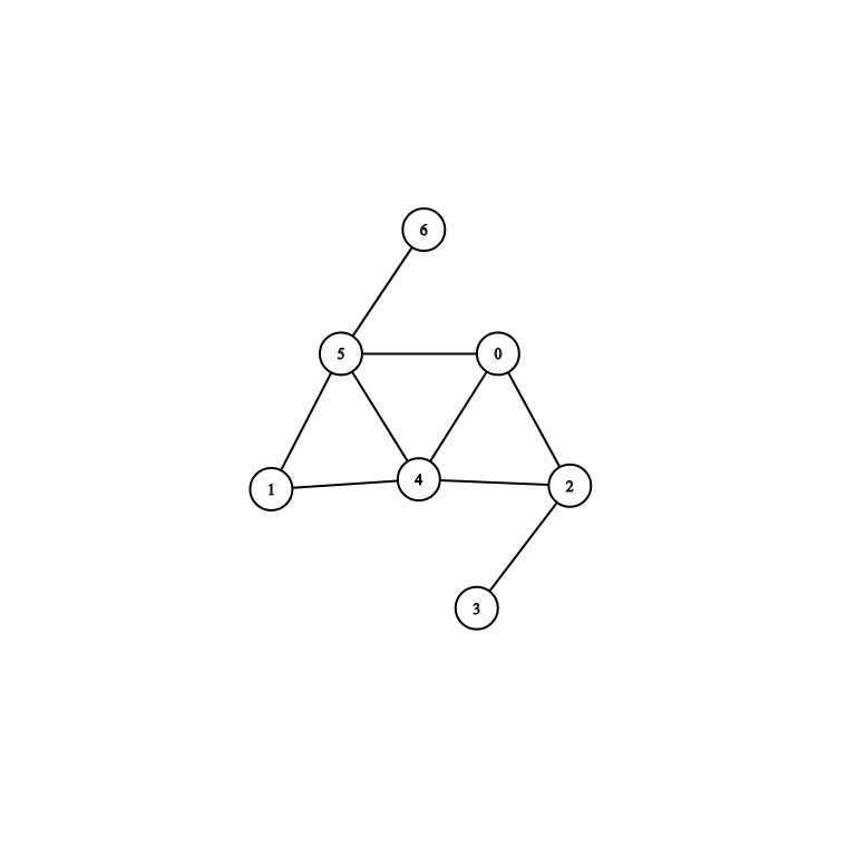
Here is the way how we can represent the graph below in edge lists fashion:

var unweightedEdgeLists = [
    [0, 4],
    [0, 5],
    [0, 2],
    [1, 4],
    [1, 5],
    [2, 3],
    [2, 4],
    [4, 5]
]

Simply we write down 2 vertices of an edge of this graph into an array which are enclosed by the array which contains all the edges.

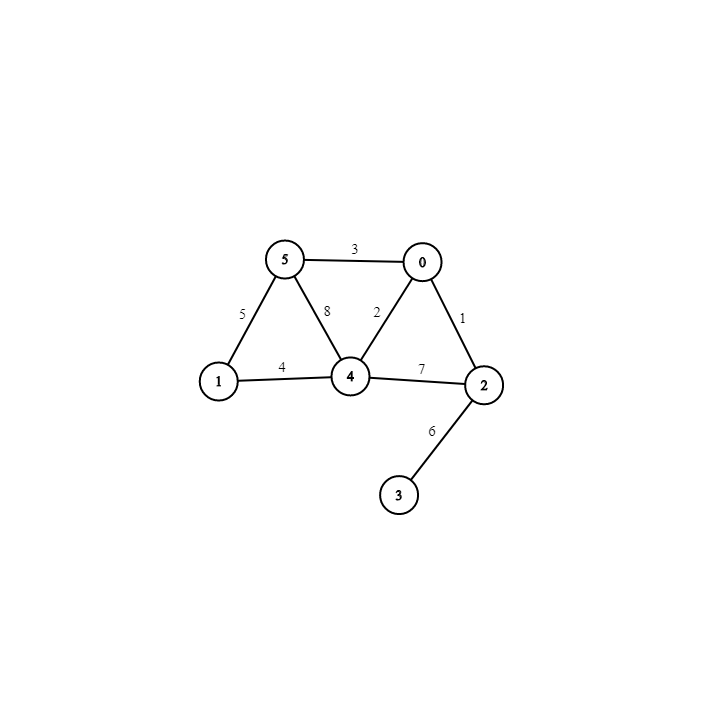
Or in this particular example above, this is a weighted graph, we do the same thing like the way we did with unweighted graph but just need to add the third element in each sub-array to represent that each edge has the weight:

var weightedEdgeLists = [
    [0, 4, 2],
    [0, 5, 3],
    [0, 2, 1],
    [1, 4, 4],
    [1, 5, 5],
    [2, 3, 6],
    [2, 4, 7],
    [4, 5, 8]
]

Edge lists are simple, but if we want to find whether the graph contains a particular edge, we have to search through the edge list. If the edges appear in the edge list in no particular order, that’s a linear search through vertical bar edges. Which leads us to learn about two other ways of graph representation below.

Adjacency matrices

Here is another way to represent a graph, which is adjacency matrix. We simply just count the total vertices and write down the $V * V$ matrices (V is a set of finite vertices). The adjacency matrices for an undirected graph is symmetric like the one you will see underneath. We list all the vertices in $V$ rows and $V$ in columns where the entry in row i and column j, we put 1 only when this graph contains an edge (i, j), otherwise, we put 0 to the corresponding position:

	0	1	2	3	4	5	6
0	0	0	1	0	1	1	0
1	0	0	0	0	1	1	0
2	1	0	0	1	1	0	0
3	0	0	1	0	0	0	0
4	1	1	1	0	0	1	0
5	1	1	0	0	1	0	1
6	0	0	0	0	0	1	0

Or you can also represent it in a particular language, such as JavaScript:

var adjacencyMatrices = [
    [0, 0, 1, 0, 1, 1, 0],
    [0, 0, 0, 0, 1, 1, 0],
    [1, 0, 0, 1, 1, 0, 0],
    [0, 0, 1, 0, 0, 0, 0],
    [1, 1, 1, 0, 0, 1, 0],
    [1, 1, 0, 0, 1, 0, 1],
    [0, 0, 0, 0, 0, 1, 0]
]

This kind of representation, adjacency matrices is predominant when compared with edge lists with respect to the time to find out whether a given edge is in the graph or not by looking up the corresponding matrix. With an adjacency matrix, we can find out whether an edge is present in constant time. We can query whether edge (i,j) is in the graph by looking at adjacencyMatrices[i][j]== 1 or not, for example, let’s choose two vertices which are 0 (as i) and 2 (as j), we know there is an edge between two vertices by looking up the table above.

But there are some disadvantages for this implementation because we have to list a matrix with $V * V$ elements, so it takes $V*V$ space, even if the graph is sparse (which contains just a few numbers of edges) we still have to spend many spaces for 0s and just a few edges. Look at the example below:

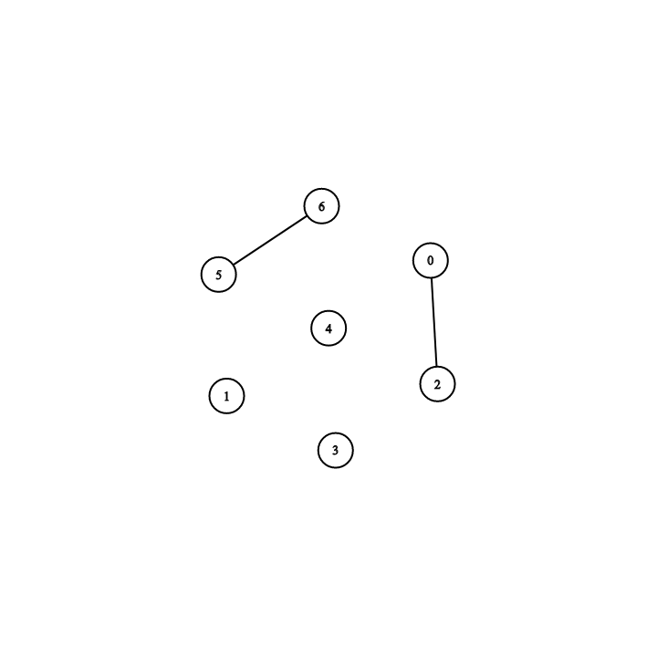
Here we just can see 2 edges in this graph, which are {0, 2} and {5,6} but if we choose adjacency matrices as our representation, it should look like this:

var sparedGraph = [
    [0, 0, 1, 0, 0, 0, 0],
    [0, 0, 0, 0, 0, 0, 0],
    [0, 0, 0, 0, 0, 0, 0],
    [0, 0, 0, 0, 0, 0, 0],
    [0, 0, 0, 0, 0, 0, 0],
    [0, 0, 0, 0, 0, 0, 1],
    [0, 0, 0, 0, 0, 0, 0]
]

And there is another disadvantage of adjacency matrices, presume that we want to find out which vertices are adjacent to a given vertex i. Like the example above, in the 6th row which is the row of vertex number 5, if we want to check how many vertices are adjacent to this vertex, we go through from begin to the end of this row, even we just found one vertex is adjected with this vertex number 5 in the last element.

Adjacency list

Adjacency lists are the combination of Edge lists and Adjacency matrices. For each vertex i in a graph, we store an array of the vertices adjacent on it (or its neighbors). We typically have an array of |V| adjacency lists, one adjacency list per vertex. Now here is one more example:

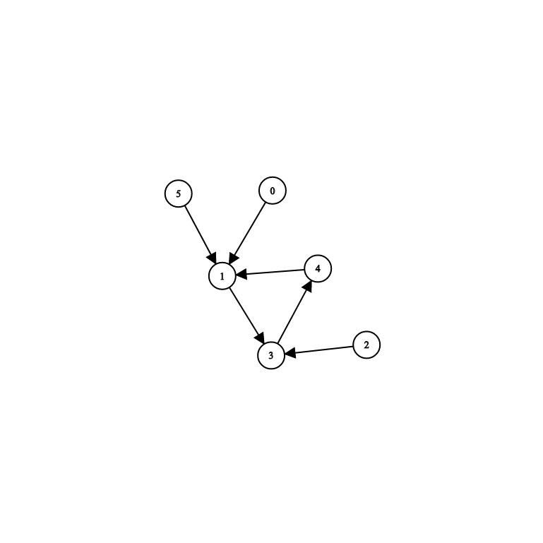
Here now we have a directed graph, and because it’s not both ways, as can be seen, so we need to represent the graph in the correct order, for example, in this image, we have an edge like this (0, 1), not like this (1, 0):

var adjancencyLists = [
    [1], // neighbor of vertex number 0
    [3], // neighbor of vertex number 1
    [3], // neighbor of vertex number 2
    [4], // neighbor of vertex number 3
    [1], // neighbor of vertex number 4
    [1] // neighbor of vertex number 5
]

With the same graph but undirected, here is how we represent this graph:

var adjancencyLists = [
    [1], // neighbor of vertex number 0
    [3, 4, 5], // neighbors of vertex number 1
    [3], // neighbor of vertex number 2
    [1, 2, 4], // neighbors of vertex number 3
    [1, 3], // neighbors of vertex number 4
    [1] // neighbor of vertex number 5
]

Adjacency lists have several advantages. For a graph with N vertices and M edges, the memory used depends on M. This makes the adjacency lists ideal for storing sparse graphs. Generally, for a directed graph, the space we need to allocate to adjacency lists is $E$ elements, for undirected graph we need $2E$ elements for this procedure because each edge $(i, j)$ appears exactly twice in the adjacency lists, once in $i's$ list and once in $j's$ list, and there are |E|edges. Let’s assume we have a directed graph with $5000$ vertices and $10000$ edges. Remember the adjacency matrices? In this case if we used adjacency matrices we had to store $5000 * 5000 = 25 000 000$ elements. Nevertheless, we just have to store 10000 $V$ vertices in case we use adjacency lists. Another advantage of adjacency lists is we can get to each vertex’s adjacency list in constant time because we just have to index into an array. In order to find a particular edge $(u, v)$ is present on the graph or not, we first need a constant time to get to the vertex $u$ then look for $v$ in $u's$ neighbors. The time we find out an edge $(u, v)$ depends upon the total vertices $u$ and the degree of this vertex. For example, we want to find an edge $(5, 10)$ , first, we need to traverse all the previous vertices until we reach the vertex number 5 then if 10 is the last vertex of this graph, we still have to traverse all of the previous vertices to get the vertex number 10 $(j)$ , but still is constant time.

Facebook0 Tweet0

Graph and its representation14 min read

Graph Description

Graph representation

Edge lists – Incident Matrix

Adjacency matrices

Adjacency list