Big O Cheat Sheet for Common Data Structures and Algorithms4 min read
When measuring the efficiency of an algorithm, we usually take into account the time and space complexity. In this article, we will glimpse those factors on some sorting algorithms and data structures, also we take a look at the growth rate of those operations.
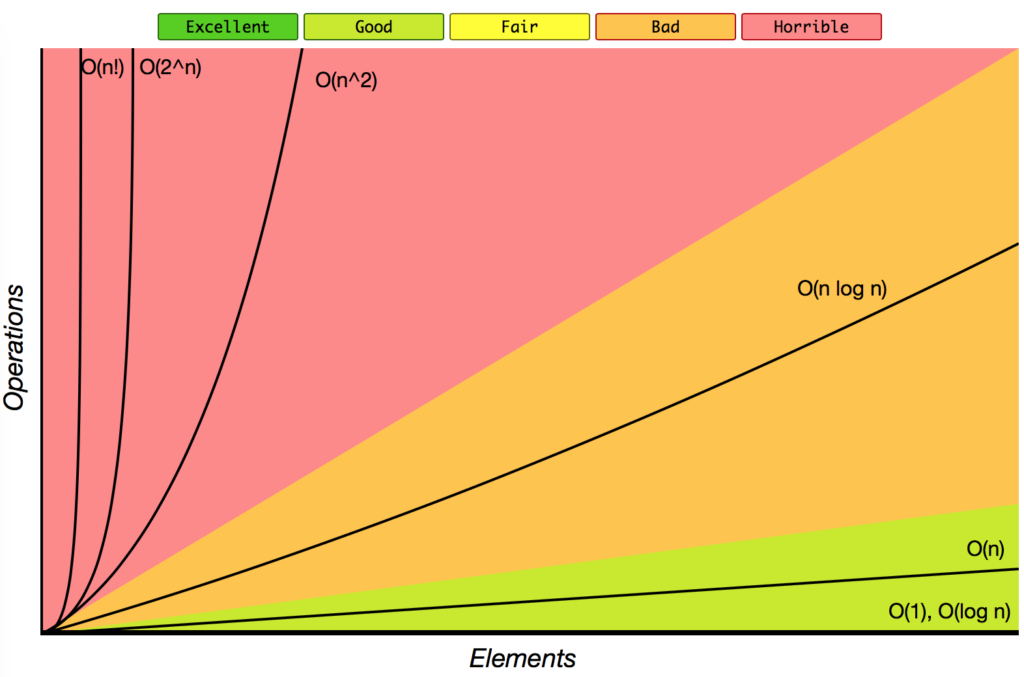
Big-O Complexity Chart
First, we consider the growth rate of some familiar operations, based on this chart, we can visualize the difference of an algorithm with O(1) when compared with O(n2). As the input larger and larger, the growth rate of some operations stays steady, but some grow further as a straight line, some operations in the rest part grow as exponential, quadratic, factorial.
Sorting Algorithms
In order to have a good comparison between different algorithms we can compare based on the resources it uses: how much time it needs to complete, how much memory it uses to solve a problem or how many operations it must do in order to solve the problem:
- Time efficiency: a measure of the amount of time an algorithm takes to solve a problem.
- Space efficiency: a measure of the amount of memory an algorithm needs to solve a problem.
- Complexity theory: a study of algorithm performance based on cost functions of statement counts.
| Sorting Algorithms | Space Complexity | Time Complexity | ||
| Worst case | Best case | Average case | Worst case | |
Bubble Sort | O(1) | O(n) | O(n2) | O(n2) |
| Heapsort | O(1) | O(n log n) | O(n log n) | O(n log n) |
| Insertion Sort | O(1) | O(n) | O(n2) | O(n2) |
| Mergesort | O(n) | O(n log n) | O(n log n) | O(n log n) |
| Quicksort | O(log n) | O(n log n) | O(n log n) | O(n log n) |
| Selection Sort | O(1) | O(n2) | O(n2) | O(n2) |
| ShellSort | O(1) | O(n) | O(n log n2) | O(n log n2) |
| Smooth Sort | O(1) | O(n) | O(n log n) | O(n log n) |
| Tree Sort | O(n) | O(n log n) | O(n log n) | O(n2) |
| Counting Sort | O(k) | O(n + k) | O(n + k) | O(n + k) |
| Cubesort | O(n) | O(n) | O(n log n) | O(n log n) |
Data Structure Operations
In this chart, we consult some popular data structures such as Array, Binary Tree, Linked-List with 3 operations Search, Insert and Delete.
| Data Structures | Average Case | Worst Case | ||||
| Search | Insert | Delete | Search | Insert | Delete | |
| Array | O(n) | N/A | N/A | O(n) | N/A | N/A |
| AVL Tree | O(log n) | O(log n) | O(log n) | O(log n) | O(log n) | O(log n) |
| B-Tree | O(log n) | O(log n) | O(log n) | O(log n) | O(log n) | O(log n) |
| Binary SearchTree | O(log n) | O(log n) | O(log n) | O(n) | O(n) | O(n) |
| Doubly Linked List | O(n) | O(1) | O(1) | O(n) | O(1) | O(1) |
| Hash table | O(1) | O(1) | O(1) | O(n) | O(n) | O(n) |
| Linked List | O(n) | O(1) | O(1) | O(n) | O(1) | O(1) |
| Red-Black tree | O(log n) | O(log n) | O(log n) | O(log n) | O(log n) | O(log n) |
| Sorted Array | O(log n) | O(n) | O(n) | O(log n) | O(n) | O(n) |
| Stack | O(n) | O(1) | O(1) | O(n) | O(1) | O(1) |
Growth of Functions
The order of growth of the running time of an algorithm gives a simple characterization of the algorithm’s efficiency and also allows us to compare the relative performance of alternative algorithms.
Below we have the function n f(n) with n as an input, and beside it we have some operations which take input n and return the total time to calculate some specific inputs.
| n f(n) | log n | n | n log n | n2 | 2n | n! |
|---|---|---|---|---|---|---|
| 10 | 0.003ns | 0.01ns | 0.033ns | 0.1ns | 1ns | 3.65ms |
| 20 | 0.004ns | 0.02ns | 0.086ns | 0.4ns | 1ms | 77years |
| 30 | 0.005ns | 0.03ns | 0.147ns | 0.9ns | 1sec | 8.4×10¹⁵yrs |
| 40 | 0.005ns | 0.04ns | 0.213ns | 1.6ns | 18.3min | — |
| 50 | 0.006ns | 0.05ns | 0.282ns | 2.5ns | 13days | — |
| 100 | 0.07 | 0.1ns | 0.644ns | 0.10ns | 4×10¹³yrs | — |
| 1,000 | 0.010ns | 1.00ns | 9.966ns | 1ms | — | — |
| 10,000 | 0.013ns | 10ns | 130ns | 100ms | — | — |
| 100,000 | 0.017ns | 0.10ms | 1.67ms | 10sec | — | — |
| 1’000,000 | 0.020ns | 1ms | 19.93ms | 16.7min | — | — |
| 10’000,000 | 0.023ns | 0.01sec | 0.23ms | 1.16days | — | — |
| 100’000,000 | 0.027ns | 0.10sec | 2.66sec | 115.7days | — | — |
| 1,000’000,000 | 0.030ns | 1sec | 29.90sec | 31.7 years | — | — |
