What is BigO Notation and Time Complexity?

When you try to solve a problem on some online websites, you probably come across some terms like BigO notation, O(n), O(1), O(n²), etc… or time complexity a couple of times, especially when solving a coding problem. So what do they mean and what are they used for?

Why Use The Term “Time Complexity”?

The same problem can be solved by different algorithms with different efficiency. To compare the efficiency of algorithms we measure it by something called computational complexity which indicates how much effort is needed for an algorithm.

If we don’t use computational complexity as a degree to measure the efficiency of an algorithm, instead we use some measurements such as millisecond or nanosecond it doesn’t work that way because you have an algorithm and it runs really fast on a computer A but it’s radically slow in computer B, an algorithm you write that is extremely fast when on C, C++ but it’s too slow when running on Python or JavaScript, if an algorithm has complied, then it is much faster than when it is interpreted, and there are a lot of other factors including processor, main memory, etc…which define the run time of an algorithm. For all these reasons, we shouldn’t use system-dependent techniques to measure the efficiency of an algorithm. That is why we need to learn and measure the efficiency of the algorithm by the computational complexity instead.

Time Complexity and Space Complexity

When trying to solve a problem, from writing flowchart to writing actual code, sometimes we can solve this problem by more than one way, it usually perhaps has several ways to solve. Hence, understanding the time complexity and also space complexity to compare the performance of different algorithms and choose the best one for a particular problem is crucial.

In computer science, the time complexity is the computational complexity that measures or estimates the time taken for running an algorithm.
Time complexity is commonly estimated by counting the number of elementary operations performed by the algorithm, supposing that an elementary operation takes a fixed amount of time to perform. In short, the time complexity of an algorithm quantifies the amount of time taken by an algorithm to run as a function of the length of the input. Time complexity is described in terms of the number of operations required instead of actual computer time because of the difference in time need de for different computers to perform the same operations. In the same way, space complexity is much like time complexity, we can define space complexity as the amount of space or memory taken by an algorithm run as a function of the length of the input. However, in the scope of this article, we just focus on time complexity.

In real cases, time and space complexity depends on many factors such as hardware, processor, memory, etc…But we don’t consider these cases for evaluating the algorithms, we just only consider the execution time for the algorithm.

Big O notation

If we want to calculate the growth of functions, knowing some concepts of discrete mathematics or calculus is essential if you want to use correct terms for calculating time complexity, but in the scope of this article, we won’t talk about calculus, you don’t have to absorb weird math concepts, instead, you still can get the general idea of how those notations look like.

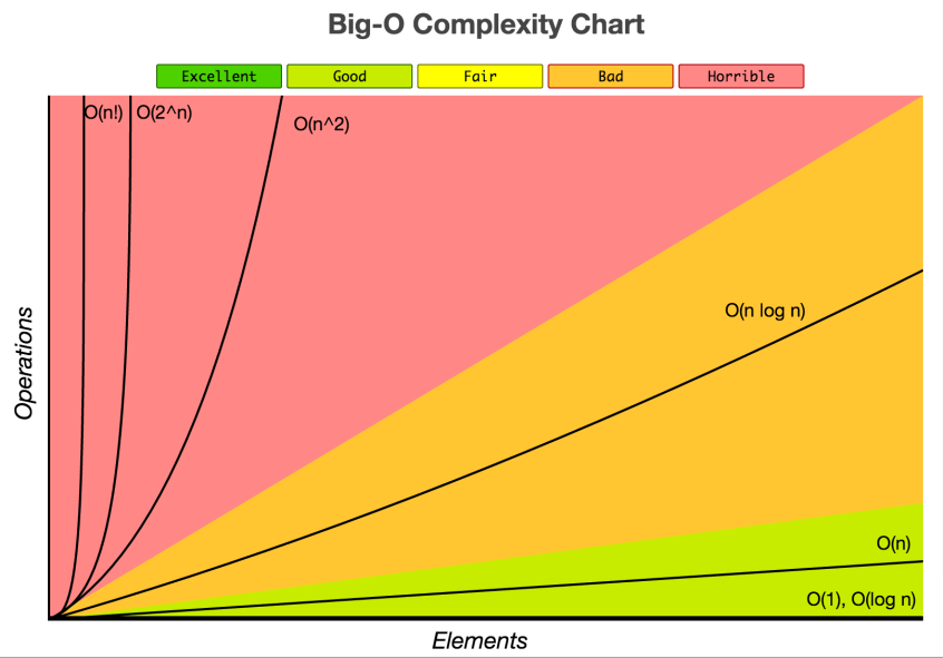
When measuring the efficiency of an algorithm as the input size becomes larger, we usually express the rate of growth by some terms such as Big-θ (pronounced Big-theta) or Big- Ω (Big-omega) and some others.

Simply speaking, Big-θ it has asymptotically tight bound whose the growth of the running time is ‘sandwiched’ between the lower bound and the upper bound on the size of a function $f\left(x\right)$ , which means Big-θ is the combination between Big-O (which will be introduced below) and Big- Ω (big-Omega) – if we just want to give a lower bound on the size of a function $f\left(x\right)$ .

In this article, we talk more about Big O notation, which is introduced underneath.

Big O (Big-Oh) notation in computer science is used to describe the worst-case scenario in a particular algorithm in terms of time complexity and/or space complexity such as execution time or the space used. Or you can say the maximum amount of time taken on inputs of a given size, which is Big O notation.

But strictly speaking, in computer science, big O notation is used to classify algorithms according to how their running time or space requirements grow as the input size grows. Big O notation characterizes functions according to their growth rates: different functions with the same growth rate may be represented using the same O notation.

The letter O is used because the growth rate of a function is also referred to as the order of the function. A description of a function in terms of big O notation usually only provides an upper bound on the growth rate of the function. Associated with big O notation are several related notations, using the symbols o, Ω, ω, and Θ, to describe other kinds of bounds on asymptotic growth rates as mentioned above.

Nevertheless, for simplicity, we often talk about Big-O notation when describing the time complexity of the algorithm, with the understanding of Big-θ would provide us more information.

O(n)

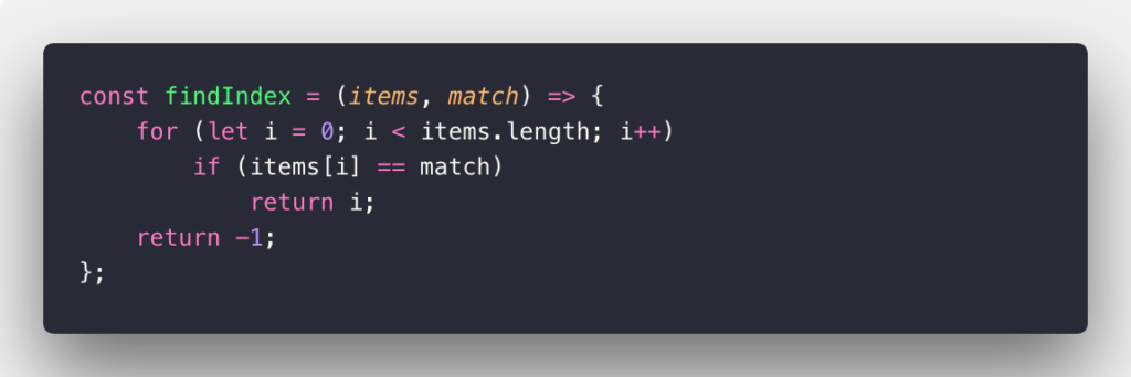
O(n) is used to describe an algorithm whose performance will grow linearly and in direct proportion to the size of the input data set (which means its graph is a straight line). The very common example for O(n) scenario is a for loop, the running time increases at most linearly with the size of the input. This example below will denote O(n) worst-case in JavaScript language:

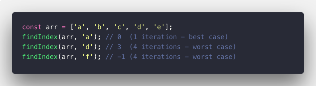
It’s more clear with the example cases below:

O(1)

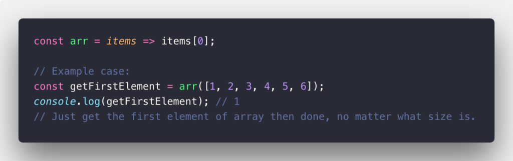
O(1) Constant time: Given an input of size n, it only takes a single step for the algorithm to accomplish the task regardless of the number of items. Consider the example below:

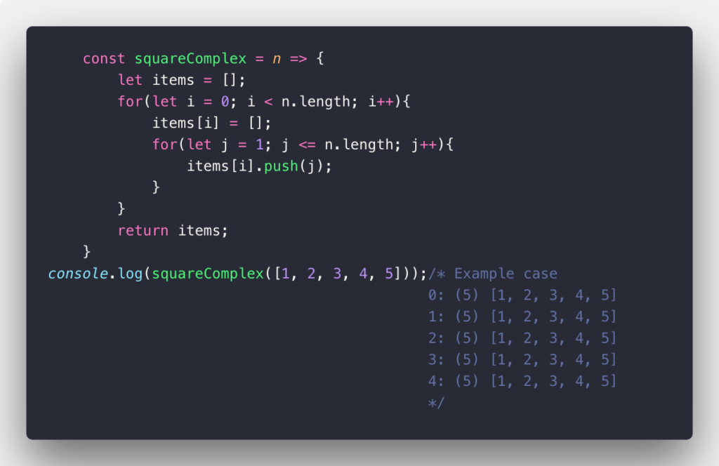
O(n²)

In this case, O(n²) also called Quadratic time is used to describe an algorithm whose performance is directly proportional to the square of the size of the input data set. This is common with algorithms that involve nested loops. Deeper iterations will lead to O(n³), O(n&sup4;), O(n&sup5;) and so on…: A common sorting algorithm like the bubble sort, selection sort, and insertion sort runs in O(n²). Take a look at the example below:

k^n and O(n!)

$k^n$ – Exponential time denotes an algorithm whose growths as exceptionally huge each input of the data set, this is common in situations when you traverse all the nodes in a binary tree. It usually exists in a recursive function, calculating Fibonacci number is one of those:

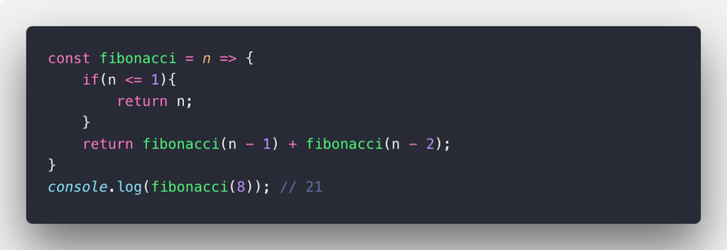
Recursive functions are usually inefficient in both memory and space complexity. So choosing recursive when there are no better ways. There is a better way to find the n-th Fibonacci number, check out this link.

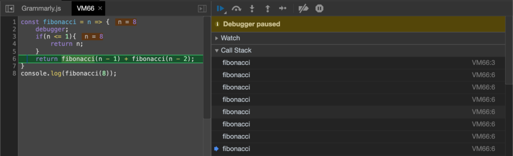
You can contemplate this code by opening up the debug mode in Chrome:

O(n!) – the factorial time is common in generating permutation:

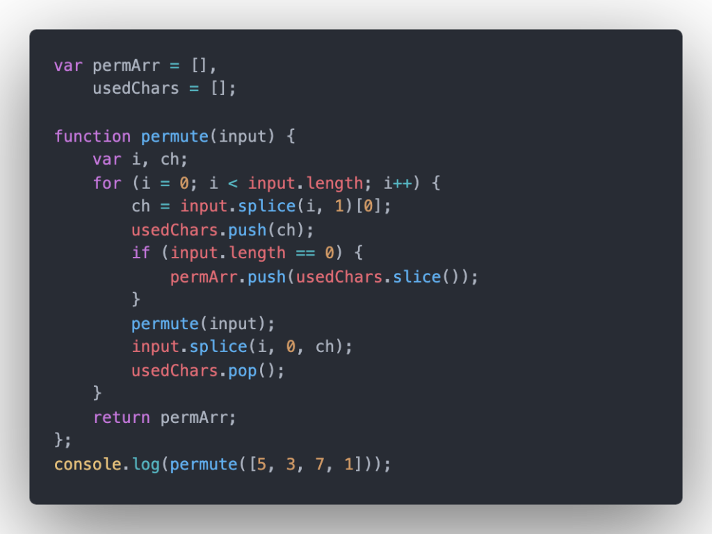
The code output:

[ [ 5, 3, 7, 1 ]
  [ 5, 3, 1, 7 ],
  [ 5, 7, 3, 1 ],
  [ 5, 7, 1, 3 ],
  [ 5, 1, 3, 7 ],
  [ 5, 1, 7, 3 ],
  [ 3, 5, 7, 1 ],
  [ 3, 5, 1, 7 ],
  [ 3, 7, 5, 1 ],
  [ 3, 7, 1, 5 ],
  [ 3, 1, 5, 7 ],
  [ 3, 1, 7, 5 ],
  [ 7, 5, 3, 1 ],
  [ 7, 5, 1, 3 ],
  [ 7, 3, 5, 1 ],
  [ 7, 3, 1, 5 ],
  [ 7, 1, 5, 3 ],
  [ 7, 1, 3, 5 ],
  [ 1, 5, 3, 7 ],
  [ 1, 5, 7, 3 ],
  [ 1, 3, 5, 7 ],
  [ 1, 3, 7, 5 ],
  [ 1, 7, 5, 3 ],
  [ 1, 7, 3, 5 ] ]

O(log N) and O(n logn)

This case is a little bit hard to explain, but in a whole, O(log N) – Quasilinear time: in many cases, the n log n running time is simply the result of performing an O(log n) operation n times. It works by selecting the middle element of the data set, essentially the median, and compares it against a target value. If the values match it will return success.
The common technique using O(log N) is the binary search or looking up a number in a phone book when you keep breaking the binary tree or phone book (which are already sorted) into 2 smaller equal sub-arrays. Begin with the interval of the whole array (binary tree, phone book) if the value of the middle equals to the value you want to find, oh yeah, just return this value and the time complexity is the best scenario with a constant time O(1), however, if the value is less than the middle then you narrow the interval in the left half, otherwise, if the value is larger than the midst, then narrow it to the right half. Keep repeating this process until finding this value or the interval becomes empty.

Also, the average case of quicksort, heapsort, and merge sort run in O(n log n) time. Look and consider the example about Quick Sort Algorithm below:

How do I define when it is O(n), O(1), O(n²)?

The time complexity of an algorithm depends on the total operations of this algorithm on given input size, please take a look at this article for more detail about time complexity and how to calculate it. But generally, there are some handy rules that you can apply to remember easier. But you can also calculate manually by yourself if you learned Discrete Math.

General Rule #1: Return statements, initialize a variable, increment, assigning, etc. All of these operations take O(1) time.
General Rule #2: The running time of the loop is at most the running time of the statements inside the loop multiplied by the number of iterations.
General Rule #3: The total running time of the nested loops is the running time of the outer loop multiplied by the inner loop(s).

Facebook0 Tweet0

What is BigO Notation and Time Complexity?10 min read